1. The Foundations of Deep Learning and Generative AI¶

Objectives

Explain the distinctions between artificial intelligence, machine learning and deep learning, and what makes a model generative
Describe how neural networks learn, from single neurons and MLPs to loss functions, backpropagation and optimisation
Justify splitting data into training, validation and test sets to detect overfitting
Recognise which generative model families (autoencoders, diffusion models, LLMs, vision-language models) are used for which life-science applications

The following notes support Session1_Intro_to_DL_Workshop.ipynb.

Deep Learning, Machine Learning and AI¶

The terms deep learning, machine learning and artifical intelligence are often used interchangeably, but they are not actually the same.

Artificial intelligence (AI) refers to any system capable of mimicking human intelligence - depending on your definition of “human intelligence”, a pocket calculator could be classed as AI. Machine learning refers to techniques where a computer learns patterns and behaviour from data rather than being explicitly programmed with every rule. Deep learning is the subset of machine learning which deals with neural networks specifically.

So deep learning is one part of machine learning, and machine learning is one part of artificial intelligence. When you hear people talk about state-of-the-art AI (especially generative AI), they usually mean deep learning. This doesn’t mean that all deep learning is generative, or that all generative AI is deep learning - but for this workshop, we’ll focus our discussion on deep learning and applications of generative neural networks to the life sciences.

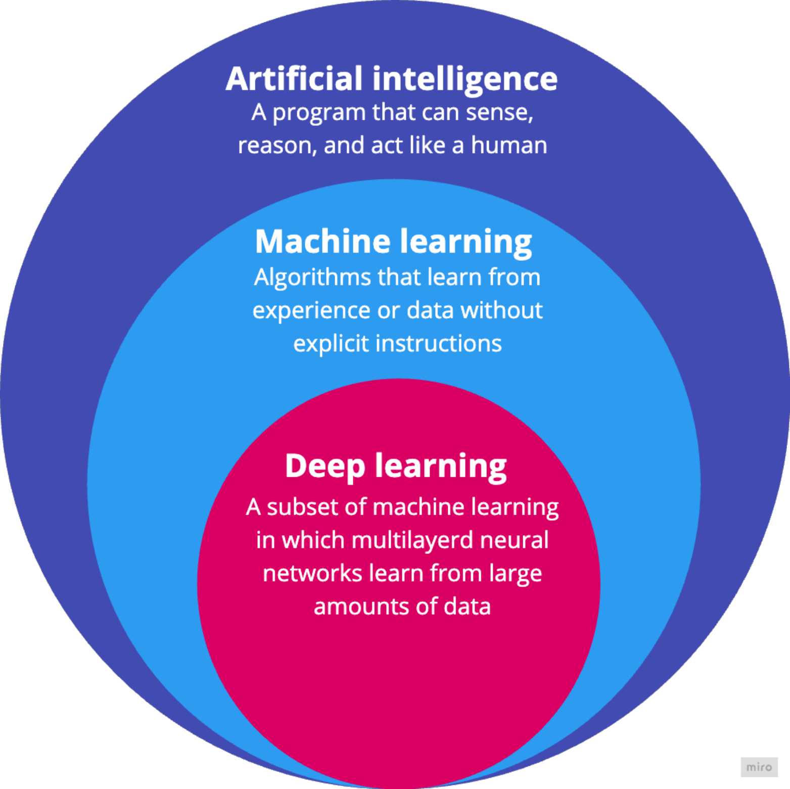
../../_images/session1_ai_ml_dl.png — A diagram showing artificial intelligence as the broadest circle, machine learning as a subset inside it, and deep learning as a subset inside machine learning.¶

The useful thing about neural networks is that they are universal function approximators. In plain English, this means that a large enough neural network can learn to approximate almost any relationship between an input and an output, as long as we give it enough data and train it properly. The network may never learn the true underlying relationship, but it can learn a useful numerical approximation.

For example, if the input is an X-ray of the lungs and the output is a diagnosis, the network could learn a function which maps from image pixels to a class label (e.g. “healthy” or “diseased”). The task of mapping input data to a categorical label is known as classification - we’ll see an example of this in Session 2.

What is Generative AI?¶

Generative AI refers to any kind of AI that can learn the patterns in data well enough to create or complete new examples. The output may be text, an image, a protein molecule, or any other quantifiable object. State-of-the-art generative AI relies almost exclusively on complex neural networks - we’ll discuss some examples in the following sections.

By now, most people have heard of GenAI systems such as ChatGPT, Claude and Gemini, which can produce fluent text and images from prompts. These commercial systems often get a bad reputation because public examples can feel gimmicky, unreliable or disconnected from real-world needs.

However, the same ideas that let models generate text, images or video also underpin scientifically valuable models with real clinical and biological applications, such as exploring disease features, helping researchers reason about complex data, and predicting protein structures or behaviour. In this workshop, we’ll see how to adapt concepts from generative AI to further meaningful research.

Why Generative AI Matters for Life Science¶

Life-science data are often high-dimensional, noisy, expensive to collect and difficult to label. Generative models are useful because they can learn patterns from the data, which can then be used for reconstruction, simulation, and interpretation.

Some examples include:

Image restoration and inpainting: improving resolution, denoising microscopy or medical images, and filling in missing image regions while preserving plausible biological structure.
Protein structure prediction: models such as AlphaFold3 use deep learning to predict protein structures from amino acid sequence information, which offers new insights into protein function and interactions.
Drug discovery: generative models can propose candidate molecules, optimise molecular properties and help explore chemical spaces too large to search manually.

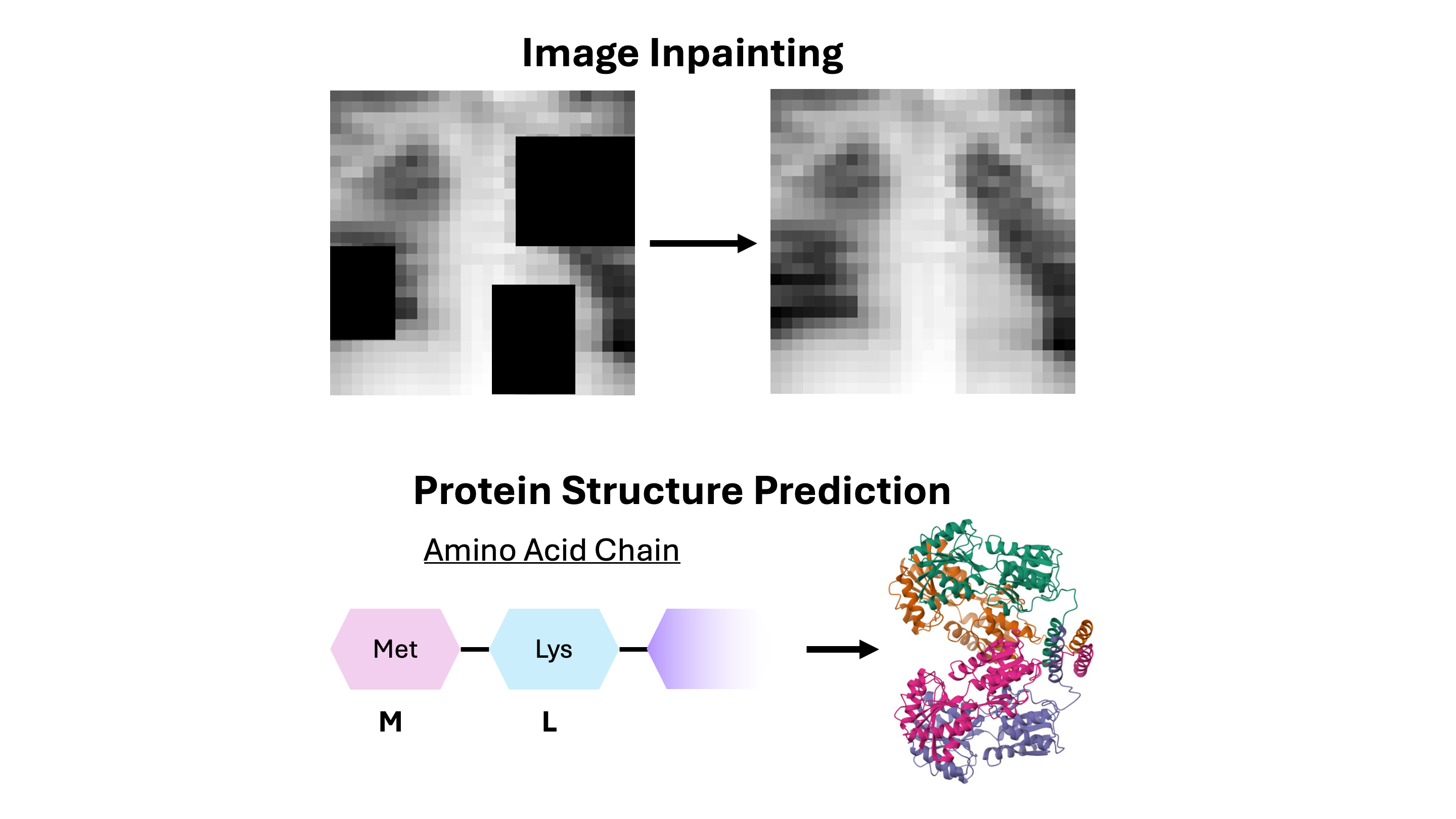
../../_images/session1_genai_life_science_applications.png — Applications of generative AI in life science.¶

Generative models are not automatically correct, but they can learn useful representations of biological variation and help researchers explore hypotheses that would otherwise be too large or expensive to test directly.

Types of Generative Models Used in Life Science¶

Several families of generative models appear repeatedly in life-science applications. We will not implement all of them in this workshop, but it is useful to know what they are and how they differ.

Autoencoders (AEs) learn to compress an input into a smaller representation (called a latent representation) and then reconstruct the original input. This forces the network to learn important features of the data. AEs are useful for denoising, dimensionality reduction, and learning interpretable latent spaces. In the first notebook, we’ll see how to implement a simple autoencoder and generate our own synthetic images.

Diffusion models generate clean data from noise. During training, real data are corrupted step by step with noise - the model then learns how to remove that noise. At generation time, the model starts from a pure noise distribution and reverses the “noising” steps back into a clean sample. Diffusion models are important in image generation and are increasingly used for molecular and protein design.

Large language models (LLMs) generate and reason over text, code and structured language-like data. Commercial models like ChatGPT and Claude are examples of LLMs. In biomedical settings, they can help with literature search, report drafting, and clinical evaluation. However, they require careful validation because fluent text is not the same as correct text.

Vision language models learn information from images, including microscopy, histopathology, and radiology data, then output a text description. State-of-the-art research in generative AI looks to creating “virtual doctors”, which can automatically describe symptoms, diagnoses and treatment options from images.

A Single Neuron¶

Warning

Maths Warning The following sections contain some mathematics, which I’m using here only for technical accuracy and completeness. Our main focus, however, isn’t in the theory behind deep learning, but in the applications to generative AI, so don’t worry if it doesn’t all make sense at first glance.

Neural networks are made up of computational units called neurons. State-of-the-art neural networks can contain millions, if not billions, of individual neurons. Each neuron is essentially a tiny calculator, which performs some simple multiplication and addition.

The input to a neural network is usually a list of numbers. These numbers could represent, for example, the RGB colour values of pixels in an image.

These numbers travel through neural networks via channels, which connect adjacent neurons. Each channel has an associated channel weight and each neuron has an associated bias. The weights and biases are just numbers, usually picked randomly at first, but the network adjusts them during training. We refer to the weights and biases collectively as the model parameters.

Each neuron will typically have multiple channels going out and multiple channels coming in. This means the neuron will take multiple inputs. Each input is multiplied by its corresponding channel weight, then all values are summed, and bias is added on top.

Finally, the total sum is put through an activation function. These are usually quite simple functions, which transform the sum in some way (you can find more information on activation functions in the sections below). This gives us our output, which can then be passed to the next neuron.

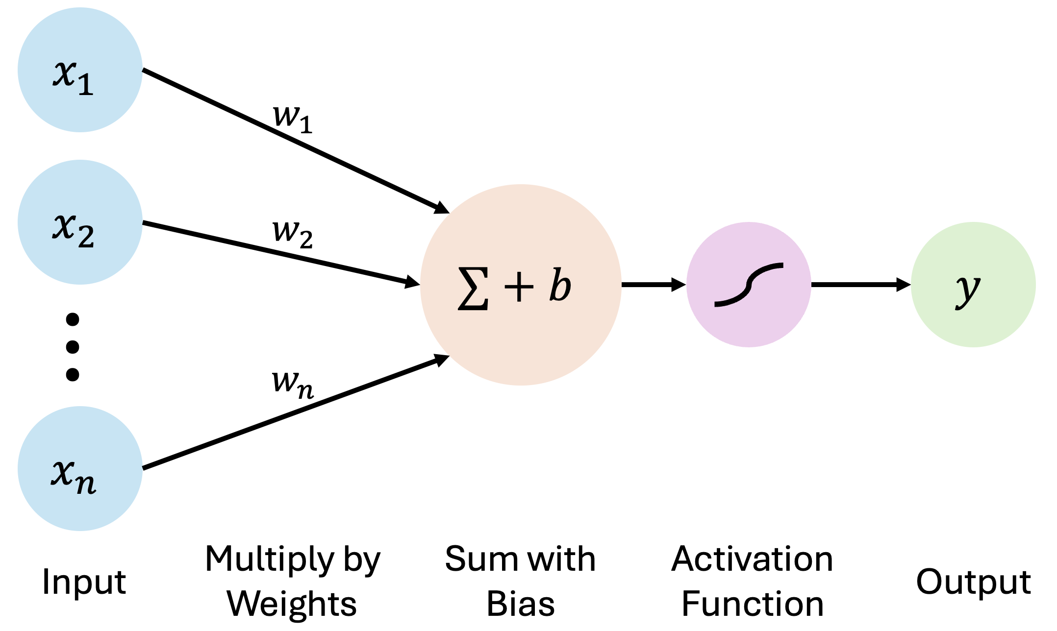
../../_images/session1_single_neuron.png — A schematic of a simple neural network. Inputs are multiplied by weights, a bias is added, and the result is passed through an activation function to produce an output.¶

To summarise, an artificial neuron takes numbers as inputs, multiplies them by learned weights, sums them, adds a bias, applies an activation function, and returns an output. We usually represent this in equation form as:

\[ y = f\left(\sum_i \left(x_i \times w_i\right) + b\right) \]

where:

$y$ is the output of the neuron.
$f$ is the activation function (you can find more information on activation functions below).
$x_i$ is an input (neurons usually take multiple inputs, e.g. $x_1$, $x_2$, $x_3$, …). The input to one neuron is usually the output of a previous neuron.
$w_i$ is the weight associated with a channel (e.g. for inputs $x_1$, $x_2$, $x_3$, we would have channel weights $w_1$, $w_2$, $w_3$).
$b$ is the bias associated with the neuron.

Let’s imagine a very simple case: suppose I have a neural network with just one neuron, and I want my network to learn to multiply every number I give it by 2. Since I have just one neuron, I would have just one weight ($w$) and one bias ($b$). Then, I could pick an activation function which does absolutely nothing (just outputs whatever input it was given). Ideally, once the network is trained, I should end up with something like $w = 2$ and $b = 0$, so for any input $x$, I get an output of $$ y = f(x \times w + b) = x \times w + b = 2 \times x $$

That may not look impressive. It is just multiply, add, transform. But now imagine doing that not once, but millions or billions of times. Suddenly the network can learn very complex relationships.

Exercise

A neuron with weights $w_1=0.5$, $w_2=1.0$ and bias $b=1$ receives inputs $x_1=2$, $x_2=3$. The neuron’s activation function is $f(x) = x$. What is the neuron’s output?

Solution

First, we calculate the weighted sum inside the neuron $0.5 * 2 + 1.0 * 3 + 1 = 5$. Passing this through the activation function gives us the output $f(5) = 5$.

We could define a single neuron in Python like this:

# Define a single neuron
def neuron(inputs, weights, bias, activation):
    # Multiply every input by its own channel weight, sum the results, then add the neuron's bias
    total = (np.asarray(inputs) * np.asarray(weights)).sum() + bias
    # Feed the total through the activation function to get the neuron's output
    return activation(total)

# The identity activation function - returns whatever it was given
def identity(x):
    return x

From Neurons to an MLP¶

Neurons are typically stacked in layers, as you can see in the figure below. A multilayer perceptron, or MLP, is the simplest kind of neural network we normally train. It is made from the following layers of neurons:

The input layer - Takes in the input data.
The hidden layers - Sit between the input and output. These layers learn intermediate representations of the data.
The output layer - Produces the final output.

MLPs are usually made up of fully-connected layers - this means every neuron in one layer is connected to every neuron in the next layer. Each connection (channel) has a weight, and each neuron has a bias. Training is the process of finding useful values for all of those weights and biases.

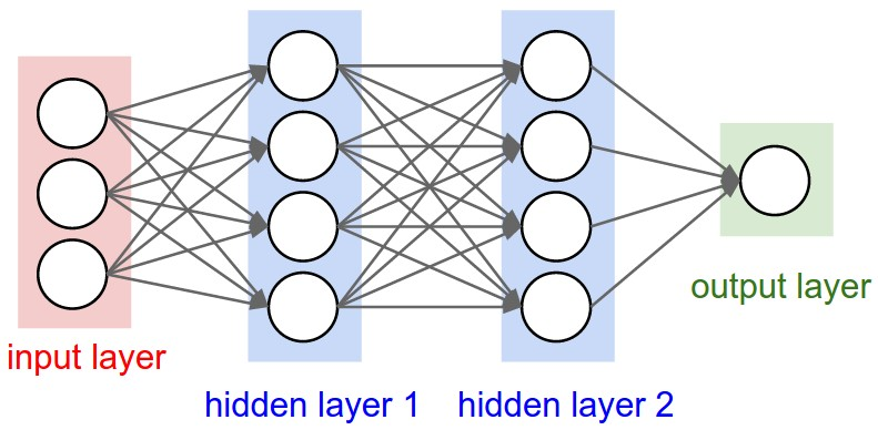
../../_images/session1_mlp_layers.png — A simple multilayer perceptron with an input layer, hidden layers and an output layer. Image source.¶

Exercise

In an MLP, a fully-connected layer maps 3 inputs to 4 neurons. How many trainable parameters does that layer have?

Solution

There are $3 * 4 = 12$ weights (one for each channel) and $4$ biases (one for each neuron). This gives $16$ parameters altogether.

This is what a simple MLP written in PyTorch looks like:

# Building a small MLP
# We can use the nn.Sequential container from PyTorch to apply each layer in the order we list them
# Each call to nn.Linear adds a new, fully-connected layer to the network
# We can also add an activation function after each layer
mlp = nn.Sequential(
    # Input layer to first hidden layer (3 inputs -> 5 neurons)
    nn.Linear(3, 5),
    # Activation function, applied to every neuron in the hidden layer
    nn.ReLU(),
    # First hidden layer to second hidden layer (5 inputs -> 5 neurons)
    nn.Linear(5, 5),
    # Another activation function
    nn.ReLU(),
    # Second hidden layer to output layer (5 inputs -> 2 neurons)
    nn.Linear(5, 2),
)

Activation Functions¶

Activation functions are what stop a neural network from creating just one big linear equation. They introduce non-linearity, which lets the network learn curved, irregular and highly complicated relationships.

Here is an example of two common activation functions:

ReLU, short for Rectified Linear Unit, returns zero for negative values and returns the input itself for positive values: $f(x)=max(0,x)$.
Sigmoid squashes values into the range 0 to 1: $f(x)=1/(1+e^{-x})$. This is good for the output layer, which may need to return binary values or probabilities, or for ensuring neuron outputs stay within a fixed range.

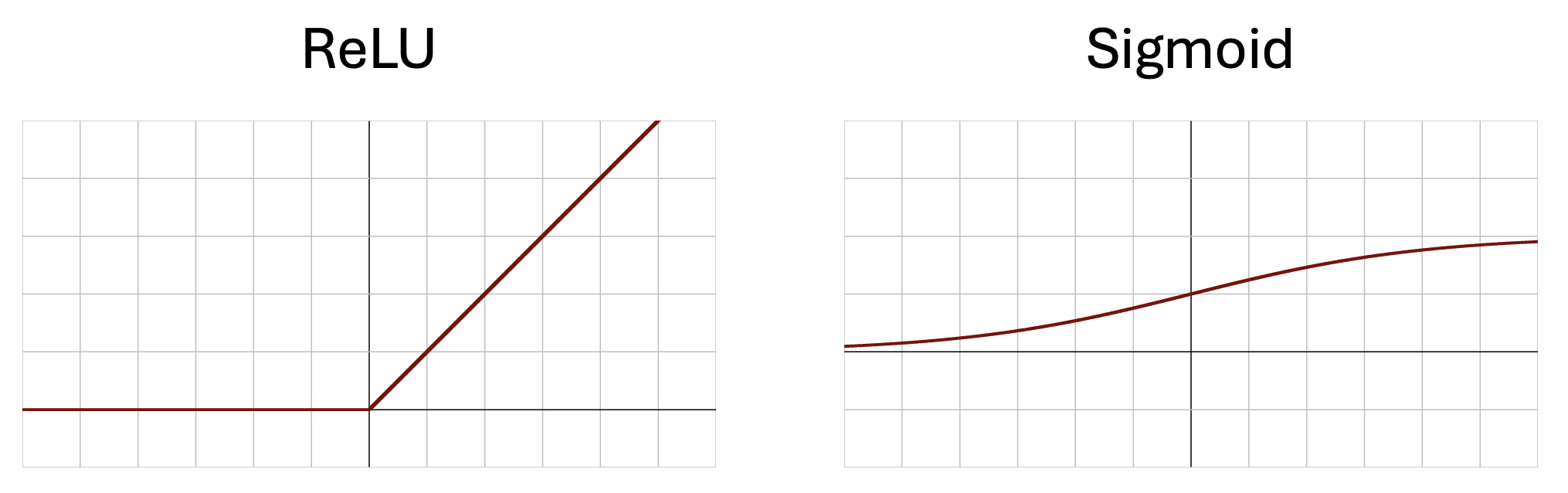
../../_images/session1_activation_functions.png — The ReLU and sigmoid activation functions.¶

Without activation functions, adding more layers would not really help. A stack of linear transformations is still just another linear transformation. ReLU, sigmoid and other activation functions let networks build non-linear curves, boundaries and representations.

In the first notebook, we’ll see the effect first-hand of adding activation functions to a neural network.

How Neural Networks Learn¶

Training means finding the model parameters (the weights and biases) that make the model’s output as close as possible to what we want. This means we need a training dataset, for which we have known input-output pairs.

Going back to our simple one-neuron example, the training dataset could contain the pairs $$(x=1, y=2), (x=3, y=6), (x=124, y=248), etc.$$ The amount of training data you need depends heavily on the model you use, but is usually in the order of 100s to 1000s of data points.

We measure “how wrong” the model is with a loss function and gradually update the model’s parameters to minimise this loss function. To do this, we must first pass our input training data through the network to get an output - this process is known as the forward pass.

The model does not know what a “good” output means, it only knows the loss we define. Typically, the loss function cannot take a negative value and has a minimum value at 0, which represents a perfect performance on the training data.

Going back to our simple one-neuron example, the loss function could be the squared error between the expected output and the output the model gave us. So, if I input the number $1$, then my expected output is $2$. Let’s say I perform a forward pass, but the model outputs $3$. Then my loss is $(3-2)^{2} = 1$. This is obviously not $0$, so my model still has some learning to do.

Once we have a loss, we need an optimiser. Optimisation is the process of adjusting the model parameters to reduce the loss. The basic idea is to work out the effect that changing the parameter (e.g. weight or bias) will have on the loss. In mathematical terms, we call this the gradient of the loss with respect to the parameters. The process of calculating the gradient of the loss with respect to the model parameters is called backpropagation.

We use a process called gradient descent to determine which direction makes the loss go up, then push the parameters in the opposite direction (i.e. to make the loss go down).

For example, in my single-neuron network, the weight of my single channel could be $3$ and the bias could be $0$. I can easily work out that increasing the weight will make my output larger, pushing it further away from the expected output of $2$ (for an input of $1$). So, I need to make the weight smaller to make the loss smaller.

The optimiser’s learning rate controls the size of each update step. If the learning rate is too small, training may be painfully slow. If it is too large, the model may jump over good solutions and become unstable.

Adam (adaptive moment estimation) is a very popular optimiser because it takes account of how each parameter has changed over time. We won’t go into too much detail here, but it’s a strong default for many neural networks.

A batch is a small group of training data processed together. Instead of calculating the loss over the entire training set before every update, we calculate it over one batch at a time. This is faster and reduces the amount of RAM (random access memory) your computer needs to use during training. One full pass through all batches in the training data is called an epoch.

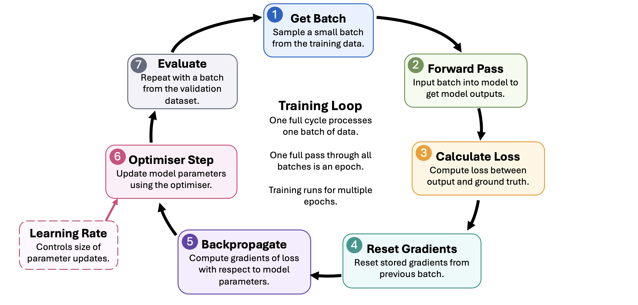
../../_images/session1_training_loop.png — The basic neural network training loop: take a batch, run a forward pass, calculate the loss, backpropagate gradients, update weights with an optimiser such as Adam, then repeat. You’ll notice there’s a seventh step, “Evaluate” - we’ll discuss that in the next section.¶

Exercise

Which of these do we learn during training and which do we choose ourselves?

Number of channels.
Channel weights.
Biases.
Learning rate.
Batch size.
Number of layers.

Solution

We choose the number of channels, learning rate, batch size and number of layers ourselves. The only learnable parameters are the weights and biases.

Train, Validation and Test Sets¶

During training, our model learns how to map the input data we provide to the expected output. However, this does not guarantee the model is learning a relationship between the input and output. A sufficiently complex model might just memorise every possible input and output pair, and completely fail on new data. This phenomenon is known as overfitting.

To mitigate this, we split our data into the following subsets:

The training set - This data is used to actually update the model parameters.
The validation set - This data is used during training to check whether the model is improving on unseen data. We usually pass this data through the model at the end of every epoch and record the loss. Note that this data is never used to update the model parameters.
The test set - This data is kept untouched until the end, giving the cleanest estimate of final performance.

If the training loss keeps decreasing but the validation loss increases, the model may be overfitting. It has learned the training examples too specifically and is no longer generalising well.

Discussion

Why do we use a test set if we already have a validation set that the model never trains on?

Solution

We use the validation loss to make decisions (when to stop training, which architecture to use), so the validation set can bias our choices. That means validation loss becomes an optimistic estimate of model performance on unseen data. The untouched test set gives the honest estimate of performance on genuinely unseen data.

A Quick Word on Tensors¶

Before a neural network can learn anything, we need somewhere to put the data. Deep learning libraries, like PyTorch, store data in tensors.

A tensor is just a container of numbers arranged in a grid. The dimension of a tensor controls how the numbers are organised:

1 dimension - a list of numbers (a vector).
2 dimensions - a table of numbers (a matrix).
3+ dimensions - a higher-dimensional array (like a stack of matrices)

We describe a tensor by its shape, which is simply the size along each dimension. By convention, the first dimension in a tensor represents the batch number. For example, the tensor $[a,b,c]$ has dimension 1 (its a vector) and shape $3$ (or $(1, 3)$ if we consider this to be a batch containing 1 vector).

There are two main reasons why we use tensors:

Speed. CPUs and GPUs are designed to work with grid-like data. We can multiply, add or transform every number in a tensor in one operation, rather than looping over them one at a time. This makes calculation much faster.
Gradients. PyTorch quietly tracks the graph of computations that led to each tensor’s calculation (which makes backpropagation much easier). Without this, we would have to differentiate the loss by hand for every parameter in the network.

A Word on Computation¶

Training a large neural network can require billions, if not trillions of parameter updates, which each require several multiplication and addition calculations of their own. As you can probably guess, this might take a very long time.

Computers typically have their own processing units, which are responsible for performing these calculations. Traditionally, abstract calculations and data processing were performed on central processing units (CPUs). CPUs are designed to handle large, complex tasks, rather than perform several small operations in parallel.

As such, training large models efficiently usually requires graphics processing units (GPUs). A GPU can perform many numerical operations in parallel, which is exactly what deep-learning workloads need. CUDA is NVIDIA’s computing platform for running general-purpose computations on NVIDIA GPUs. In practice, frameworks such as PyTorch use CUDA behind the scenes so that tensor operations, backpropagation and optimisation can run much faster than on a CPU. So, if you see “CUDA” written anywhere in the notebooks, that’s just us telling the program to run calculations on the GPU rather than CPU.

Overview of the First Notebook¶

In the first notebook, we’ll put the fundamental concepts we’ve introduced into practice. Working through the notebook, we will:

Set up our Python environment.
Explicitly define a single neuron.
Stack neurons into a multilayer perceptron (MLP).
Test a simple network with and without activation functions.
Train a network on a simple task.
Split data into training, validation and test sets, and force a model to overfit.