Anatomy of a Large Language Model
A language model does not read text as words and sentences: text must first be converted into numerical representations, then transformer layers update those representations using the surrounding context.
A simplified forward pass looks like this:
text
  -> tokens
  -> token IDs
  -> embeddings
  -> transformer blocks
  -> output logits
  -> next-token probabilities
For a generative language model, the process is repeated one generated token at a time.
Questions
How does text become input to a neural network?
What information is contained in a token embedding?
How does attention introduce context?
What do queries, keys, and values represent?
What is the role of the feed-forward layers?
Why can decoder-only models not attend to future tokens?
Objectives
By the end of this episode, learners should be able to:
describe the path from text to tokens, embeddings, and output probabilities;
explain why modern language models use subword tokenisation;
distinguish an initial token embedding from a contextual representation;
describe self-attention using queries, keys, and values;
explain the purpose of causal masking;
distinguish the role of attention from the role of a feed-forward network;
recognize the main differences between encoder-only, decoder-only, and encoder-decoder models.
From text to tokens
The first step is tokenisation. A tokeniser divides the input into units called tokens and maps every token to an integer ID.
Tokens do not necessarily correspond to words. Depending on the tokeniser, a token may represent a complete word, part of a word, punctuation, whitespace, or another frequently occurring character sequence.
Why not use one token per word?
A word-level vocabulary is simple to imagine:
"The"       -> 104
"model"     -> 527
"predicts"  -> 8912
"a"         -> 37
"token"     -> 2841
This approach soon becomes impractical. A vocabulary would need separate entries for plurals, conjugations, spelling variants, compound words, technical terms, names, and typographical errors. It would also handle languages with productive word formation poorly.
At the other extreme, a model could process individual characters. This keeps the vocabulary small, but makes sequences considerably longer. The model must then learn how characters form common words before it can learn higher-level relationships.
Modern language models usually use subword tokenisation as a compromise. Common words may remain as single tokens, while uncommon words are divided into reusable pieces.
For example, a tokeniser might represent:
supercomputing
as something conceptually similar to:
super + comput + ing
The actual split depends on the tokeniser and on the data from which its vocabulary was constructed.
Tokenisation is part of the model
A model must be used with the tokeniser with which it was trained.
Token IDs have no universal meaning. Token ID 527 may represent one token
for one model and an entirely different token for another.
Why tokenisation matters
Tokenisation affects the length of the sequence seen by the model. This in turn affects memory use, computation, and the amount of text that fits within the context window.
It can also affect performance across languages and specialist domains. A tokeniser may represent frequent English words efficiently while dividing a scientific term or a word from another language into many small fragments. The model can still process such text, but the representation uses more positions and may have been encountered less often during training.
Think like a tokenizer
Consider the following strings:
train
training
pretraining
retraining
supercomputer
supercomputing
Without using a real tokeniser, propose a possible subword vocabulary that could represent all six strings.
There is no single correct answer. Discuss the trade-off between a larger vocabulary and longer token sequences.
Solution
One possible vocabulary contains:
train
ing
pre
re
super
computer
comput
This would allow:
train          -> train
training       -> train + ing
pretraining    -> pre + train + ing
retraining     -> re + train + ing
supercomputer  -> super + computer
supercomputing -> super + comput + ing
A larger vocabulary could include every complete word, producing shorter sequences. A smaller vocabulary would reuse more pieces but produce longer sequences. Real tokenisers choose a compromise based on frequencies in their training corpus, often using an algorithm called byte-pair encoding (BPE).
From token IDs to embeddings
A token ID is an integer label. The numerical distance between two token IDs has no semantic meaning. Token ID 100 is not inherently more similar to token ID 101 than it is to token ID 9000.
Before the transformer can process the tokens, the model maps every token ID to a vector. This operation is performed by an embedding layer.
If the vocabulary contains (V) tokens and the model uses an embedding dimension (d), the embedding layer can be represented as a matrix:
Looking up a token ID selects the corresponding row of this matrix.
token ID
   |
   v
embedding matrix lookup
   |
   v
vector of length d
The embedding matrix is learned during training. Tokens that are useful in
similar contexts often acquire related representations. The number d determines
the number of dimensions in the embedding space, and since it is often large, it
can be hard to visualize. We can however project the vectors into a 2D or 3D and
draw some conclusions.
Embedding vectors and semantic similarity
Visualizing Word2Vec embeddings.
Search for the word “woman”, “boy”, “girl”, “husband”
Do you notice any patterns?
Solution
Woman and husband has approximately the same “distance” as boy and girl. We can see that the Word2Vec model has learned that gender is a meaningful dimension in the embedding space.
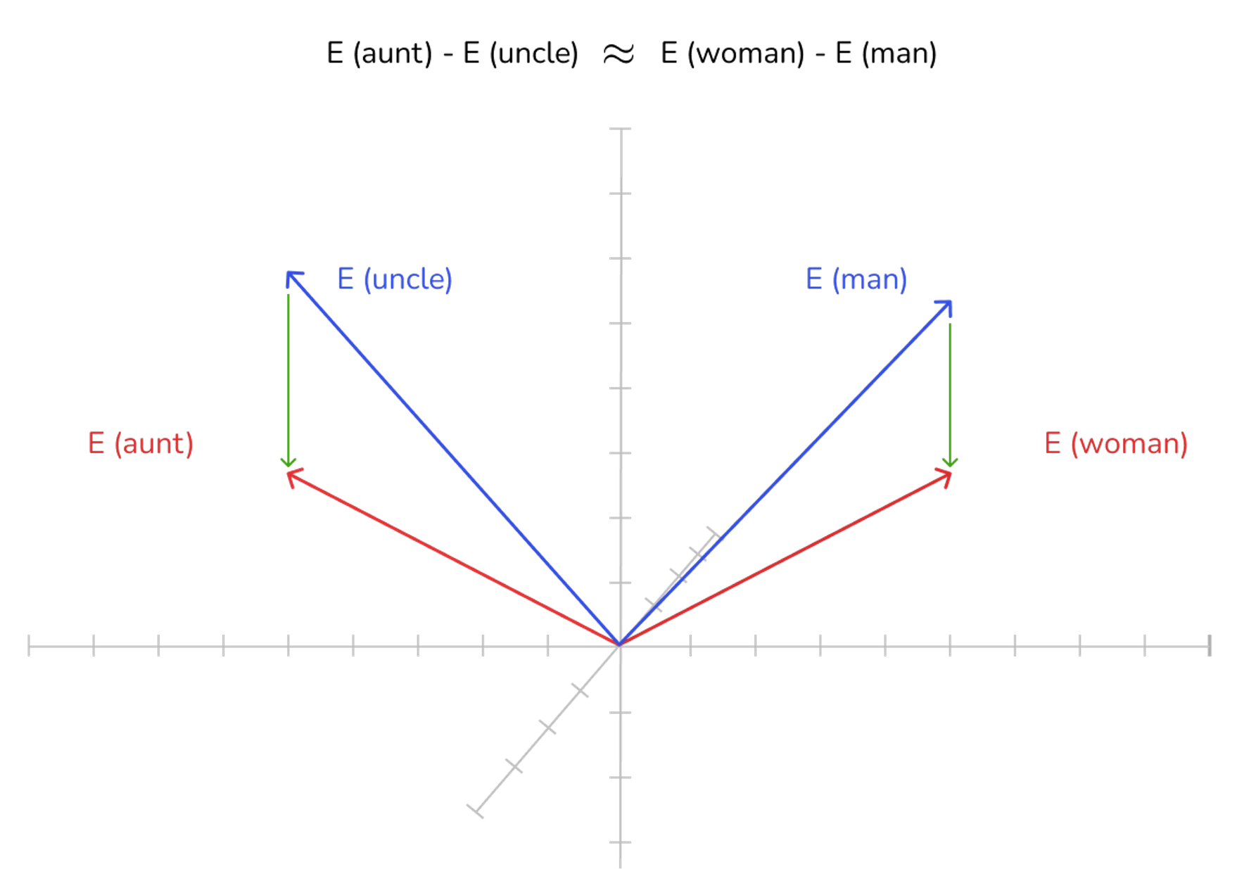
More Word2Vec
Go to https://projector.tensorflow.org/ and explore the embeddings. Click on any random word (depicted as blob), and observe and reflect on the “neighbouring” words.
Initial and contextual representations
The embedding-layer output is only the initial representation of a token. It does not yet express what the token means in a particular sentence.
Consider the word mole:
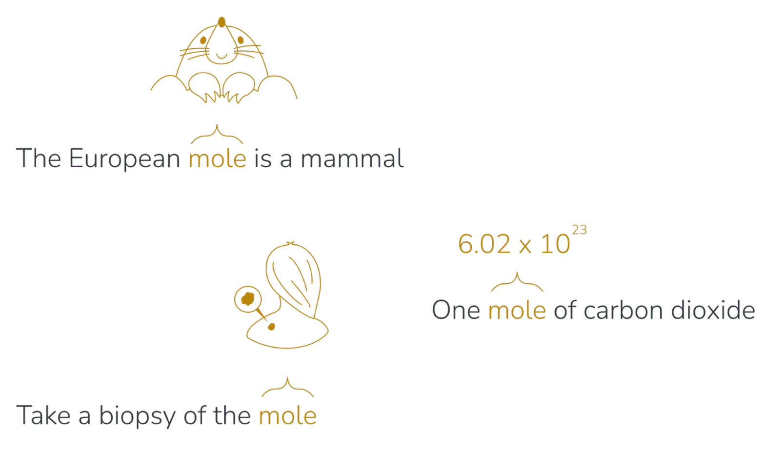
Another example for the word mole
A mole damaged the garden.
The chemist measured one mole of the compound.
She has a mole on her cheek.
The tokeniser may assign the same token ID to mole in every sentence. The
embedding lookup therefore produces the same initial vector.
The surrounding context is different, however. Transformer layers use that
context to produce a different representation of mole in each example.
The same principle applies when an expression changes meaning as context is added:
lion
sea lion
sea lion cuddly toy
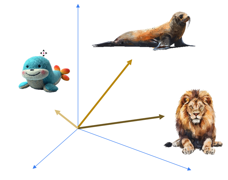
The initial vector associated with the token lion is unchanged. Its
contextual representation changes because the words around it change.
Embeddings vs contextual representations
An embedding often refers to the initial vector produced by the embedding layer, whereas a contextual representation is the vector associated with a token after one or more transformer layers have processed the sequence.
Sometimes the word embedding is used to refer to both, which can be confusing.
Important
We need a mechanism with which to encode the position, context, and the semantic meaning of each (sub-)word/token/embedding in the text. This is what the transformer architecture solves.
Type of transformers
Transformer architectures are commonly grouped into three broad families.
Encoder-only models
An encoder-only model builds contextual representations using information from both sides of a token. This is useful when the model must understand an entire input rather than generate a continuation.
Encoder-only models are commonly associated with classification, named-entity recognition, semantic similarity, and extractive question answering.
Decoder-only models
A decoder-only model predicts the next token based on the tokens that precede it. Most contemporary general-purpose generative language models use this architecture.
At each generation step, the model produces a probability distribution over the vocabulary. A decoding procedure selects a token, appends it to the sequence, and invokes the model again.
Encoder-decoder models
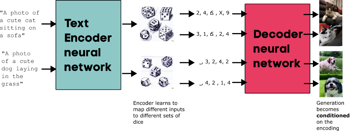
Text to image generative model as an example of an encoder-decoder model. Think DALL-E, Stable Diffusion, FLUX.1 [dev] etc..
An encoder-decoder model first builds representations of the input with an encoder. A decoder then generates an output while attending to both the already generated output and the encoded input.
This architecture is well suited for sequence-to-sequence tasks such as translation and summarization. They are also used for multimodal tasks such as image segmentation (for eg., Detectron) and generation (for eg., Stable Diffusion).
Focus of this lesson
The remainder of the episode concentrates on decoder-only models because they are the usual basis of instruction-tuned and chat-oriented language models. The main components also appear in other transformer families.
Inside a transformer block
A transformer contains a stack of repeated blocks. Although details differ between model families, each block contains two major computational components:
an attention sublayer;
a position-wise feed-forward network, often called an MLP (multi-layer perceptron).
Residual connections and normalization layers support the flow of information through the network.
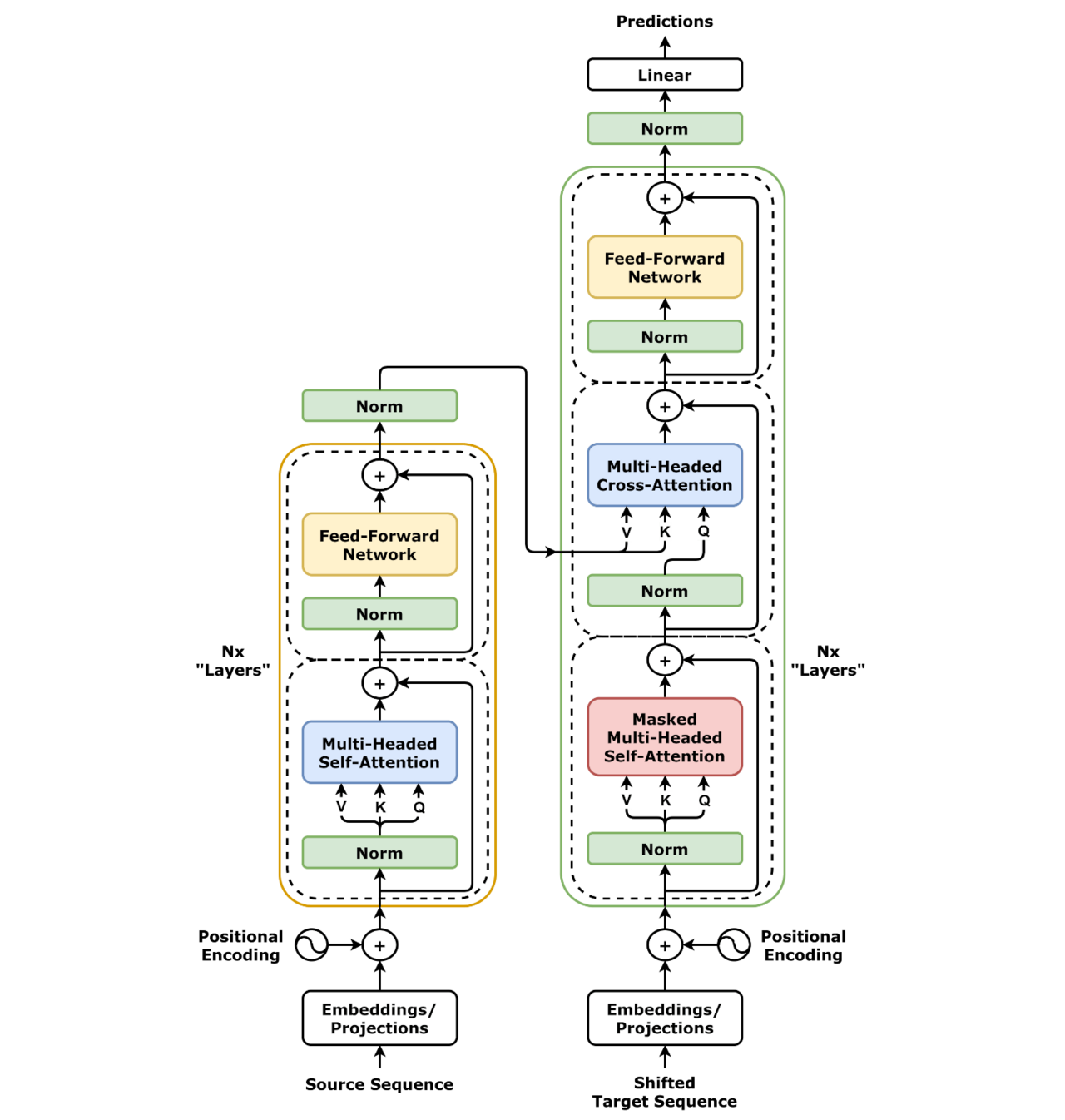
The original transformer architecture. Modern large language models often use decoder-only variants, but retain the repeated pattern of attention, feed-forward layers, residual connections, and normalization. Source

A concise conceptual distinction is:
Attention moves information between token positions.

The feed-forward network transforms the representation at each position.
Both components contain learned parameters, and both are changed during training.
Position in the sequence
Attention alone does not inherently know whether one token comes before or after another. The model must therefore include information about position.
The original transformer added positional encodings to token embeddings. Modern architectures may use other methods, such as learned position embeddings or rotary position embeddings.
The implementation differs, but the purpose is the same: token representations must contain enough positional information for the model to distinguish sequences such as:
the dog chased the cat
and:
the cat chased the dog
Self-attention
Self-attention allows the representation at one token position to incorporate information from other token positions in the same sequence.
For every token, an attention head computes three vectors:
the query describes what information the current position is looking for;
the key describes information that a position can be matched on;
the value carries information that can be passed to another position.
The vectors are produced by learned linear projections of the current token representations:
Here, \(X\) contains the input representations for all positions. The matrices \(W_Q\), \(W_K\), and \(W_V\) are learned model parameters.
Comparing queries and keys
The model computes a dot product between each query and each key. A larger dot product means that the query and key are more strongly aligned in the learned representation space.
The scaled dot-product attention operation is:
The expression can be read in three stages.
First, the model computes:
This produces a matrix of attention scores. Every row corresponds to a query position, and every column corresponds to a key position.
The scores are divided by the square root of the key dimension. Without this scaling, dot products tend to grow as the vector dimension increases, which can make the softmax operation difficult to optimize.
Softmax then converts each row into normalized weights. The final matrix multiplication uses those weights to form a weighted combination of the value vectors.
A concrete interpretation
Suppose the model processes:
The researcher deposited the data because it was required.
The representation at it needs information from the preceding context. One
or more attention heads may assign useful weight to data or to words that
help establish the relationship between it and data.
It is tempting to say that a particular head is a “pronoun head” or that another head always connects adjectives to nouns, but while it is a useful mental model, internal representations are a lot more opaque than this, which is one of the sources of the lack of interpretability of LLMs.
Another example:
The fat ginger cat sat on a mat
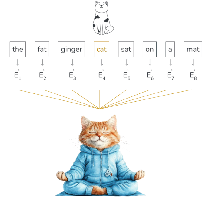
It the context contains adjectives (fat, ginger) which describes the appearance of cat
and also the verb sat and object mat which describes the position of the cat.
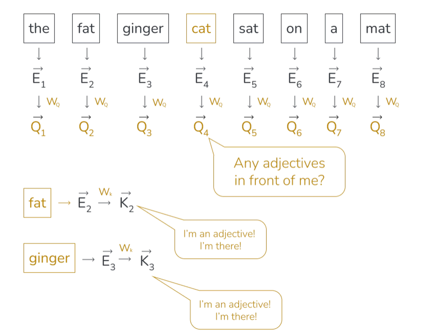
If we imagine that there exists a particular attention head which focussing on nouns. The query vector is like looking for labels with “adjective” on them to better understand the noun. In reality, this is much more abstract.
Causal masking
During next-token training, a decoder-only model must not use future tokens to predict an earlier token.
Consider:
The cat sat down
When the model predicts sat, it may use The and cat. It must not use
sat or down as input evidence for that prediction.
The model applies a causal mask to the attention scores:
             key position
             1  2  3  4
query 1      x  -  -  -
query 2      x  x  -  -
query 3      x  x  x  -
query 4      x  x  x  x
An x marks an allowed attention connection. A - marks a connection that is
masked before softmax.
Query-Key dot product
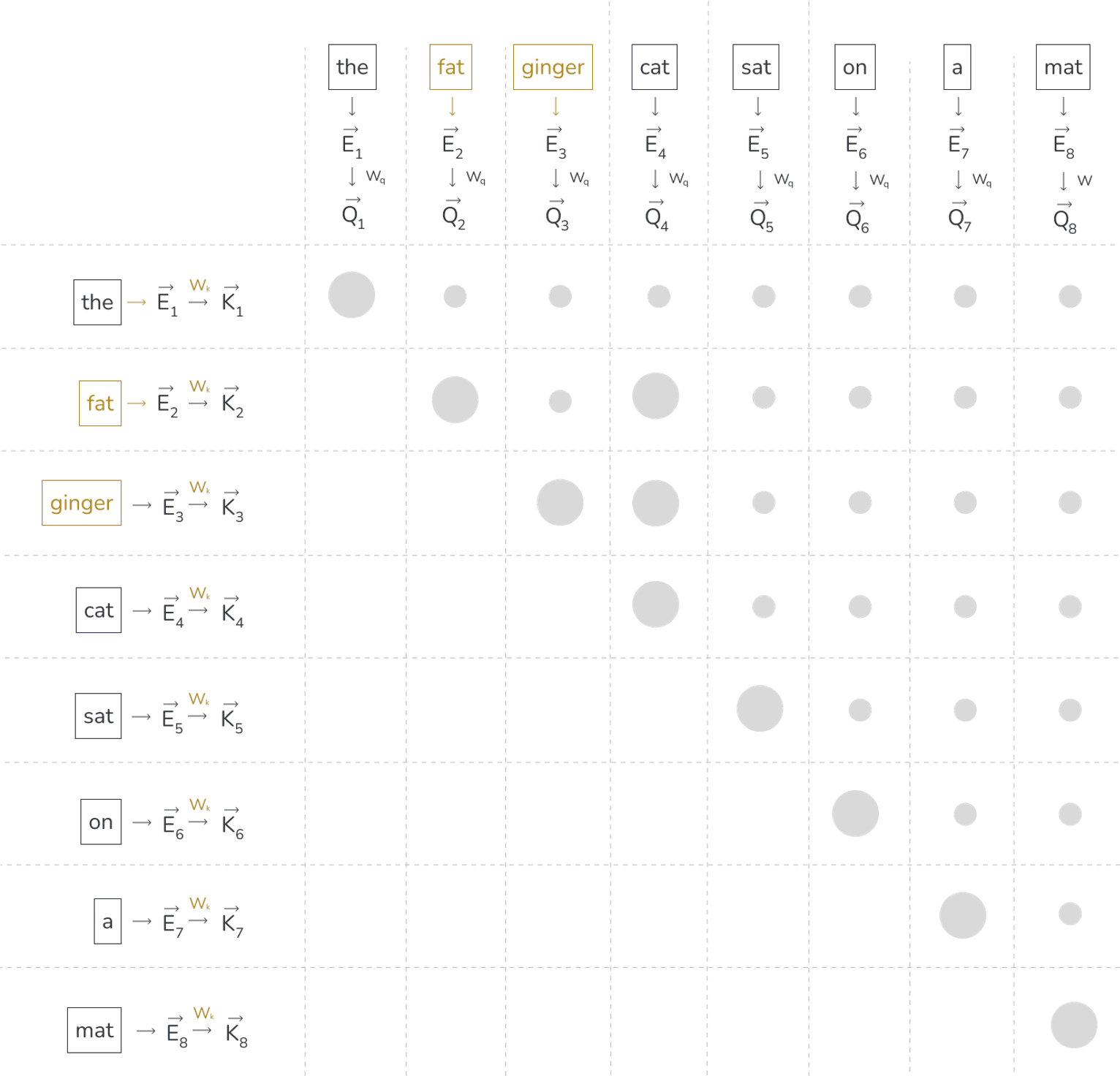
Compute the dot product with each query-key pair, to determine how well the key matches the query. Where the queries and keys align, the dot product is larger. Lower left dot products are masked, as we want the model to predict every next word during training. To prevent data leakage, future words should not influence previous ones.
During inference this is not very important (the future tokens do not exist yet), but it is essential in the training phase to prevent “cheating”.
From values to attention
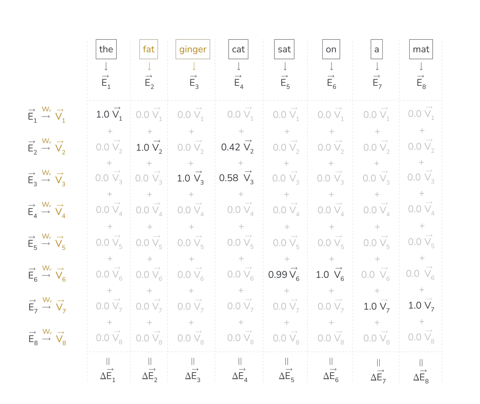
Value matrix multiplied by the embedding of the previous word results in the value vector
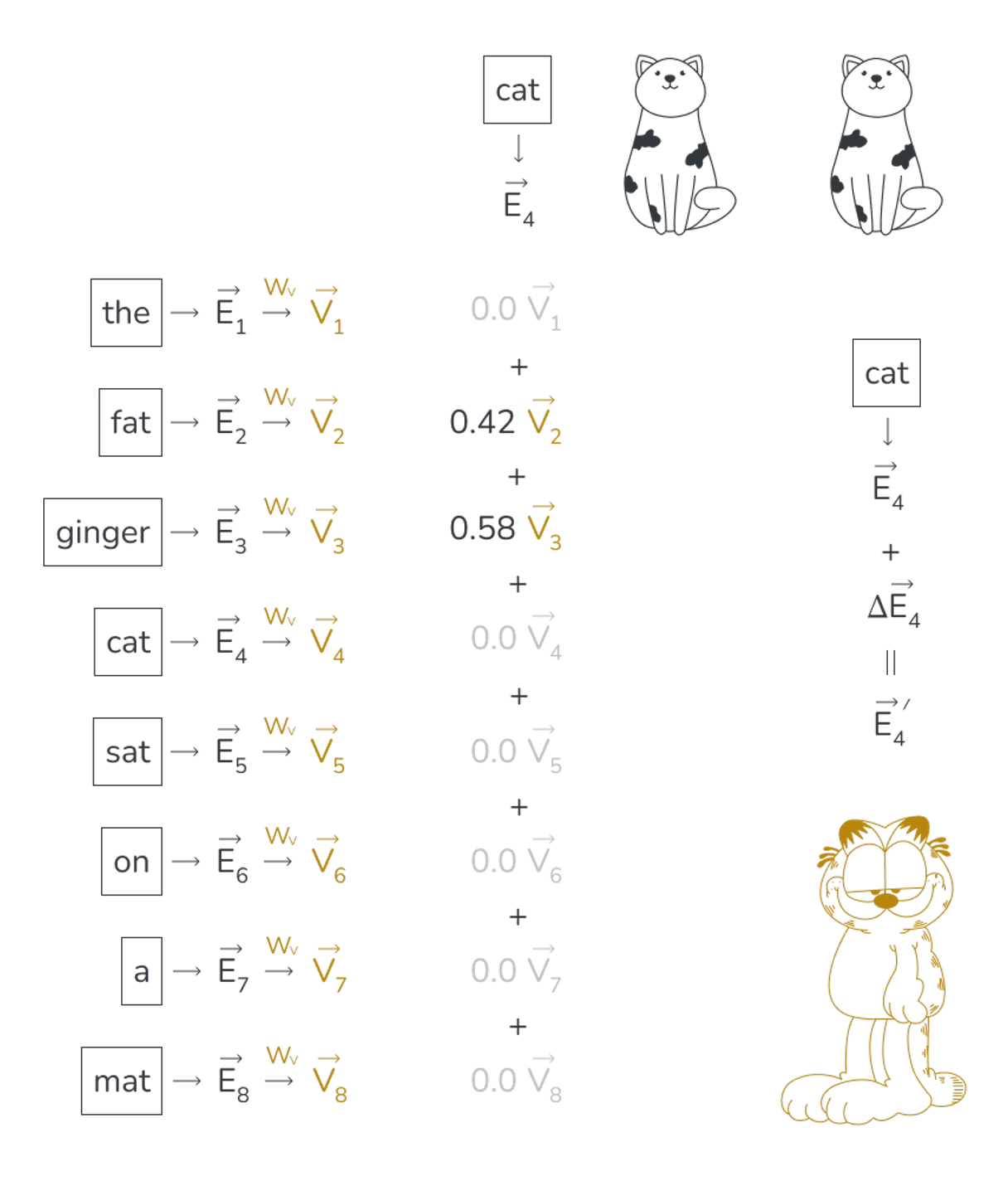
Each value vector is the multiplied by the corresponding weight and summed up to form the attention vector. This attention vector represents a “change” in the embedding to get an updated, richer meaning. Since this happens to every word in the sequences we end up with a set of more refined embeddings.
Sidenote: Context length and computational cost
For standard dense attention, a sequence containing (n) tokens produces an attention-score matrix containing (n^2) entries for every head.
Doubling the sequence length therefore produces approximately four times as many query-key comparisons. The total cost of a transformer also includes projection and feed-forward operations, so end-to-end scaling is more complicated than one formula suggests. Nevertheless, the quadratic attention matrix is an important reason why long contexts can be expensive. There are a few tricks to mitigate this, such as KV caching.
Multi-head attention
A transformer does not compute a single attention pattern. It computes several attention heads in parallel.
Each head has its own query, key, and value projections. This allows different heads to construct different patterns of information exchange. The outputs of the heads are concatenated and passed through another learned projection.
input representations
       |
       +-> attention head 1 --+
       +-> attention head 2 --+
       +-> attention head 3 --+-> concatenate -> output projection
       +->        ...         |
       +-> attention head h --+
The number of heads is an architectural choice. More heads do not simply mean that the model has a corresponding number of human-interpretable rules.
Feed-forward networks
After attention has exchanged information between token positions, a feed-forward network transforms the representation at each position.
A simplified feed-forward operation is:
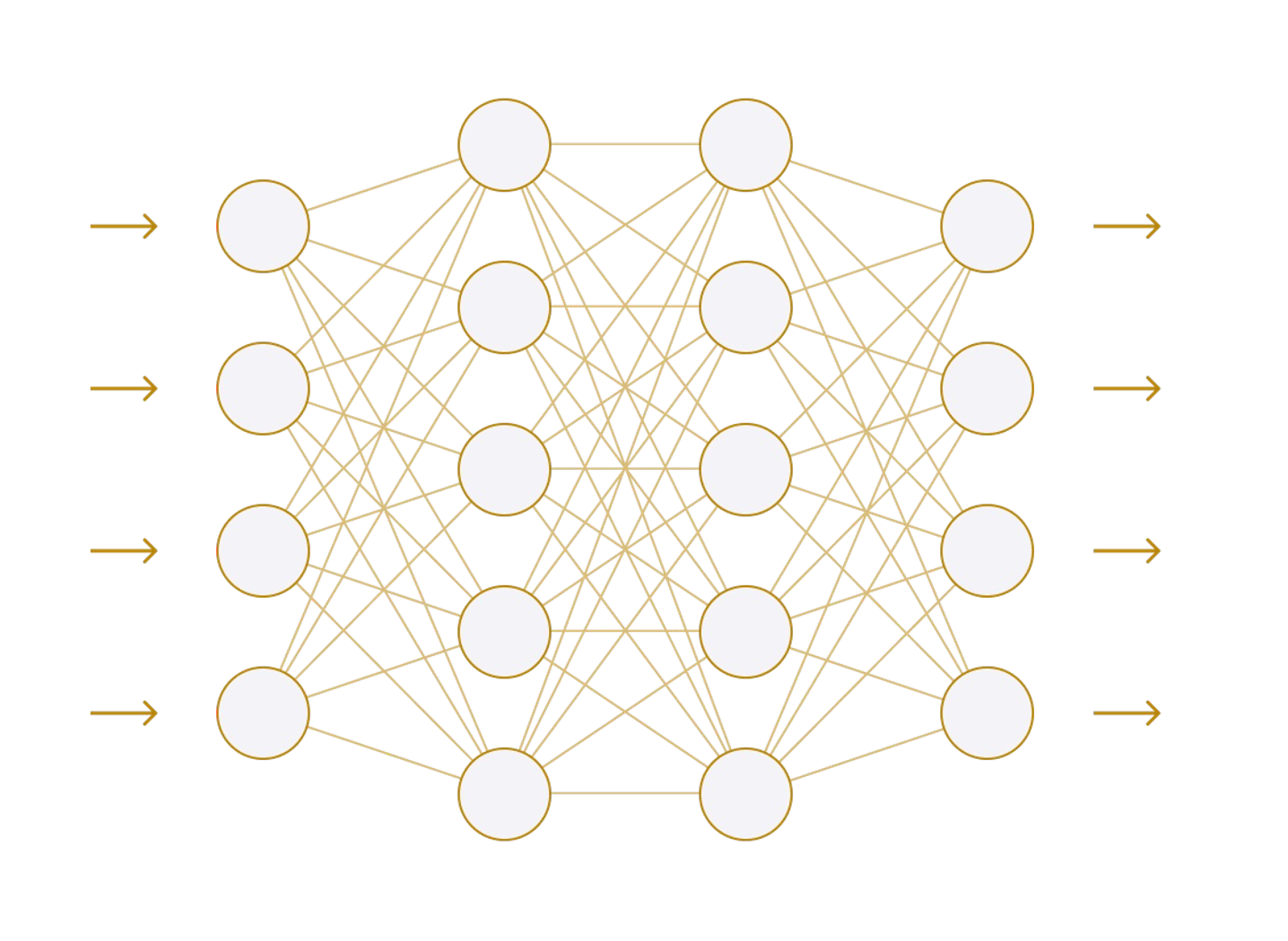
The first projection usually expands the hidden representation to a larger intermediate dimension. A nonlinear activation is applied, followed by a projection back to the model’s hidden dimension.
The same feed-forward parameters are applied independently at each token position.
token position 1 -> same feed-forward network -> updated position 1
token position 2 -> same feed-forward network -> updated position 2
token position 3 -> same feed-forward network -> updated position 3
Attention and feed-forward layers therefore perform complementary work. Attention allows positions to exchange information. The feed-forward network then performs a richer transformation of each resulting representation.
Feed-forward layers contain a large fraction of the parameters in many transformer architectures. This gives them substantial representational capacity.
Where is model knowledge stored?
It is sometimes said that attention controls context while the feed-forward layers store knowledge. This can be a useful first approximation, but it is not a precise division.
Learned associations are distributed across embeddings, attention projections, feed-forward parameters, normalization, and the interactions between layers.
Residual connections and normalization
A transformer block does not replace its input representation outright. Residual connections allow a sublayer to contribute an update:
The original representation can therefore continue through the network while each sublayer adds new information.
Normalization controls the scale of activations and makes deep networks easier to train. Different architectures place normalization before or after the attention and feed-forward operations, but its general purpose remains training stability.
From representations to token probabilities
After the final transformer block, the model converts the representation at the relevant sequence position into one score for every token in the vocabulary. These scores are called logits.
Softmax turns the logits into a probability distribution:
"the"        0.31
"a"          0.14
"this"       0.08
"model"      0.03
...          ...
A decoding strategy then selects the next token. Always choosing the most probable token is called greedy decoding. Other strategies sample from the distribution, possibly after adjusting it through temperature, top-k, or top-p sampling.
The selected token is appended to the input, and the process is repeated.
prompt
  -> predict one token
  -> append token
  -> predict another token
  -> append token
  -> continue until stopping
A fluent response is therefore constructed through repeated next-token prediction, not by producing a complete paragraph in a single operation.
Exercise: Trace information through the model
Trace a forward pass
Consider the prompt:
The experiment failed because the input file was
Describe what happens between receiving this text and producing a probability for the next token.
Your explanation should include:
tokenisation;
the embedding lookup;
positional information;
attention;
the feed-forward layers;
output logits and softmax.
Do not try to predict the exact tokeniser output or the exact next token.
exercise-forward-pass
The tokenizer divides the text into tokens and maps those tokens to integer IDs. The embedding layer maps each ID to an initial vector, and the model incorporates positional information so that token order is represented.
The vectors pass through a sequence of transformer blocks. Masked self-attention lets each position combine information from earlier positions but prevents access to future positions. Feed-forward layers transform each contextual representation independently. Residual connections and normalization support the flow of information through the blocks.
After the final block, the representation at the last input position is projected to one logit for every vocabulary token. Softmax converts the logits into probabilities. A decoding strategy selects the next token from that distribution.
Exercise: Attention and masking
Construct a causal mask
Write the causal attention mask for a sequence of five tokens.
Then answer:
How many positions can token 1 attend to?
How many positions can token 5 attend to?
Why is the mask needed during training even though the complete training sentence is already available?
exercise-causal-mask
The mask is:
             key position
             1  2  3  4  5
query 1      x  -  -  -  -
query 2      x  x  -  -  -
query 3      x  x  x  -  -
query 4      x  x  x  x  -
query 5      x  x  x  x  x
Token 1 can attend to one position. Token 5 can attend to all five positions, including itself.
The complete sentence is available during training so that predictions for many positions can be computed efficiently in parallel. Without the mask, the model could inspect the tokens it is meant to predict. That would leak the answers into the input and would not reproduce the autoregressive conditions used during generation.
Training pipeline
When a LLM is first trained, three steps are usually involved:
Pretraining: the model is trained on large unstructured corpora of text, in an unsupervised manner, just trying to predict the next token. This is what gives origin to the base models, which understand language constructs and syntax.
Supervised fine-tuning (SFT): the model is trained on question-answer pairs, possibly with reasoning traces. This is when model are actually trained to perform a task (coding assistant, chat interface, etc.) and produces the so-called “instruct” models.
Reinforcement/alignment training: the model is trained using reinforcement learning techniques, like DPO and GRPO, to influence its alignment to human values and teach it how to reply in a way that better reflects human preferences. After this it is usually ready to ship.
The fine-tuning that is the subject of this course is, essentially, a repetition of step 2.
Summary
A language model begins by dividing text into tokens. Token IDs are mapped to initial vectors, and positional information records where those tokens occur in the sequence.
Transformer blocks repeatedly update the representations. Attention exchanges information between token positions. Queries and keys determine which positions are relevant, while values contain the information that is combined. Causal masking prevents a decoder-only model from using future tokens.
Feed-forward layers transform each contextual representation independently. Residual connections and normalization make it possible to train a deep stack of these operations.
Finally, the model converts the last representation into logits and then into a probability distribution over the vocabulary. Text generation repeats this next-token prediction process until a stopping condition is reached.